2026-07-08 TRITC On-chip Urea Assay — Blank-subtracted Analysis

Optical setup: 4× objective + 1.5× zoom, TRITC bandpass filter (~530–590 nm), 0.987 µm/px.

Calibration: 0, 0.5, 1, 2, 5, 10, 15, 20 mM urea. Unknowns: 0.75, 3, 7, 12, 17 mM urea. All solutions from the same stock in the same chip.

Analysis method

With a 0 mM urea standard, the assay becomes cleanly framed as a blank-subtracted, path-length-normalised colorimetric measurement. The 0 mM standard captures the baseline color of the full assay mixture under the same mixing, timing, imaging, and device conditions as the urea samples.

A 0 mM urea standard was processed identically to the urea-containing samples and used as the assay blank. For each sample, absorbance was computed at each channel height and blank-subtracted height-by-height. The blank-subtracted absorbance was then fit as a function of path length, yielding a slope (Δm) that served as the path-length-normalised assay signal. Urea concentration was determined from a calibration curve relating Δm to known urea concentration, while the linearity of ΔA versus path length provided an internal Beer–Lambert quality-control check.

Absorbance: A_i(c) = −log₁₀(T_i(c))
Blank subtraction: ΔA_i(c) = A_i(c) − A_i(0 mM)
Fit ΔA vs path length: ΔA_i = Δb + Δm × l_i
Calibration curve: Δm vs c_urea
Predict unknowns: c = (Δm_unknown − Δm₀) / S

1. Blank-subtracted absorbance (ΔA) matrix

ΔA_i(c) = A_i(c) − A_i(0 mM) for each section and non-zero concentration.

	S1	S2	S3	S4	S5	S6	S7	S8
Concentration
0.5mM	-0.00079	-0.00067	-0.00064	-0.00053	-0.00041	-0.00033	-0.00031	-0.00028
1mM	0.00213	0.00158	0.00131	0.00093	0.00091	0.00075	0.00064	0.00038
2mM	0.00531	0.00415	0.00357	0.00274	0.00242	0.00241	0.00160	0.00121
5mM	0.02448	0.01980	0.01734	0.01382	0.01193	0.01031	0.00828	0.00670
10mM	0.06101	0.04882	0.04198	0.03314	0.02757	0.02155	0.01804	0.01477
15mM	0.09139	0.07302	0.06256	0.04911	0.04074	0.03154	0.02615	0.02056
20mM	0.11366	0.09059	0.07747	0.06053	0.05021	0.03900	0.03216	0.02503

2. ΔA vs path length — calibration

Table: QC metrics for each calibration concentration. Δm is the primary assay signal; Δb should be near zero for a clean blank subtraction.

Concentration	c (mM)	dm (AU/um)	db (AU)	R2
0.5mM	0.5	-0.000003	-0.00020	0.96441
1mM	1.0	0.000010	0.00019	0.98246
2mM	2.0	0.000023	0.00081	0.97475
5mM	5.0	0.000102	0.00451	0.99240
10mM	10.0	0.000272	0.00782	0.99623
15mM	15.0	0.000415	0.01045	0.99547
20mM	20.0	0.000519	0.01245	0.99569

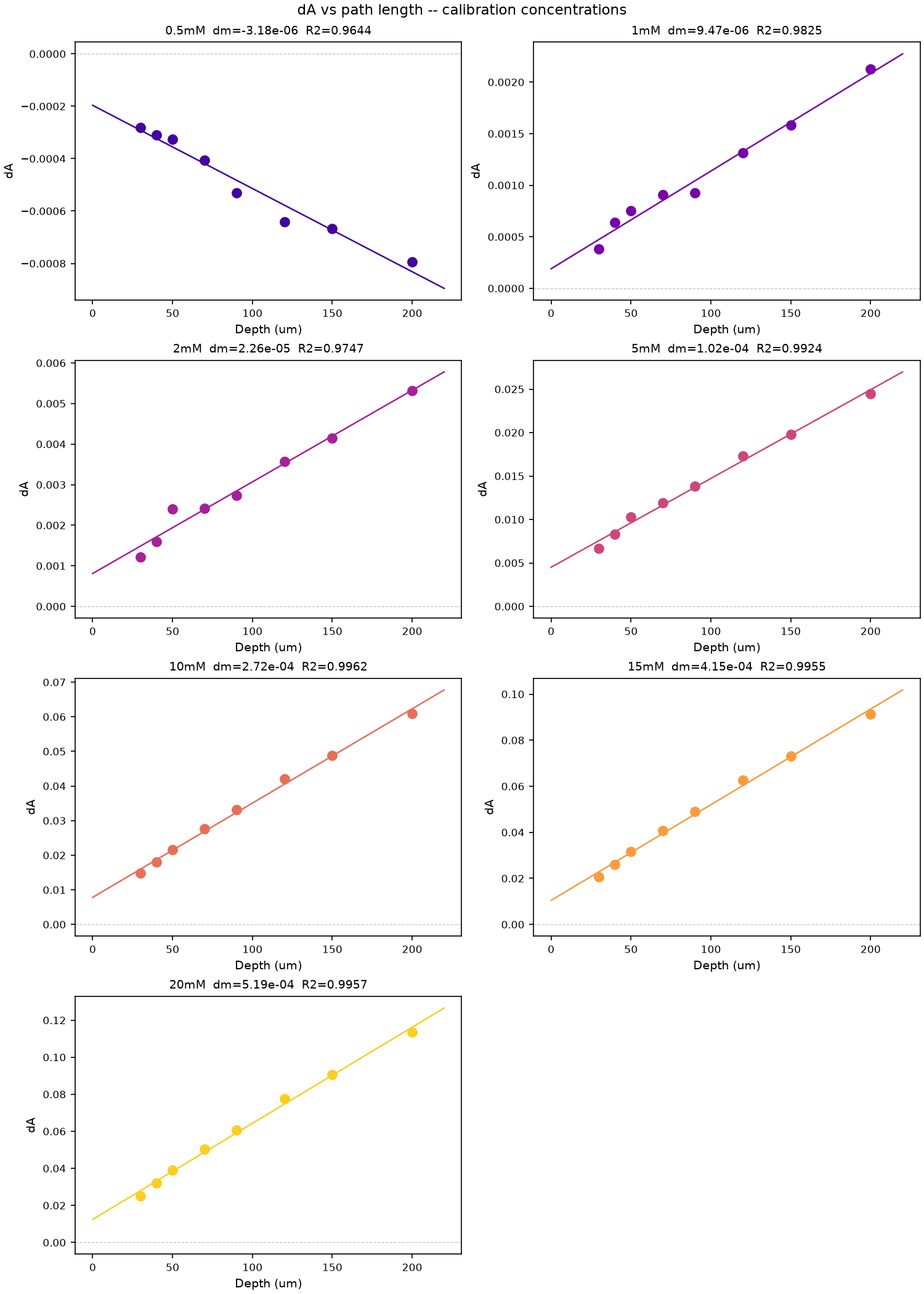
Figure 1. ΔA vs optical path length for each calibration concentration. Points: measured ΔA per section. Lines: linear fit. Good Beer–Lambert behaviour appears as points on the line with intercept near zero.

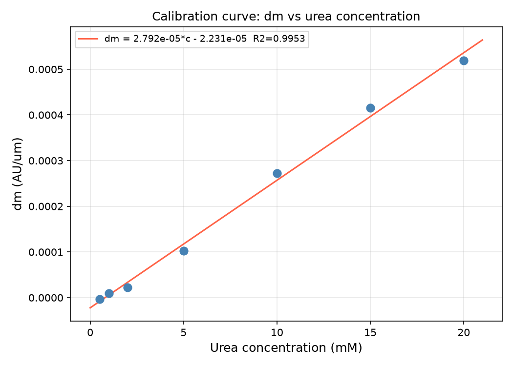
3. Calibration curve: Δm vs concentration

Figure 2. Slope Δm extracted from each ΔA vs depth fit, plotted against known urea concentration. Sensitivity S = 2.792e-05 AU/µm/mM, R² = 0.9953.

4. Unknown concentration prediction

Δm_unknown is extracted from the ΔA vs depth fit and inverted: c = (Δm − Δm₀) / S.

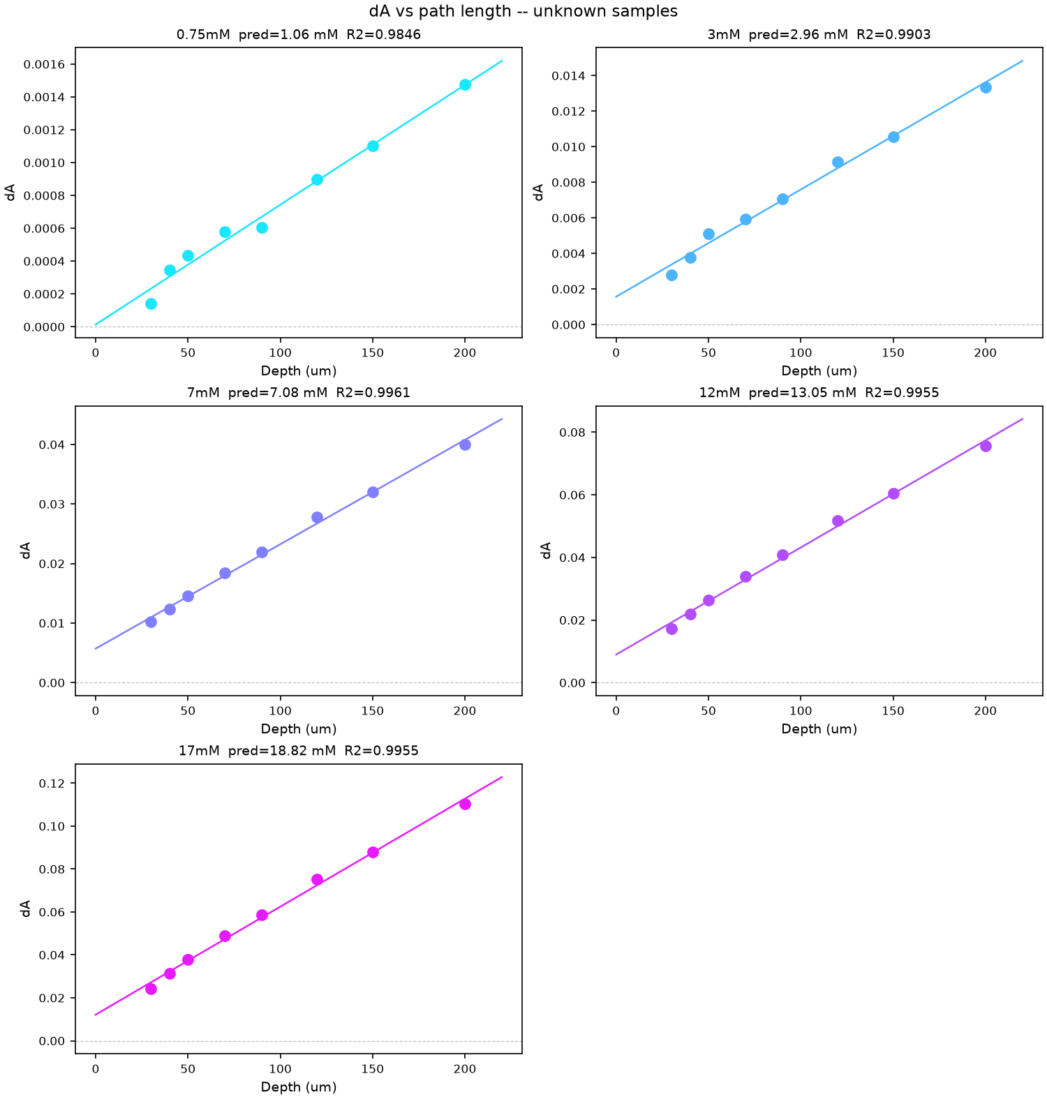
Figure 3. ΔA vs optical path length for unknown samples. Predicted concentration and R² shown in each panel title.

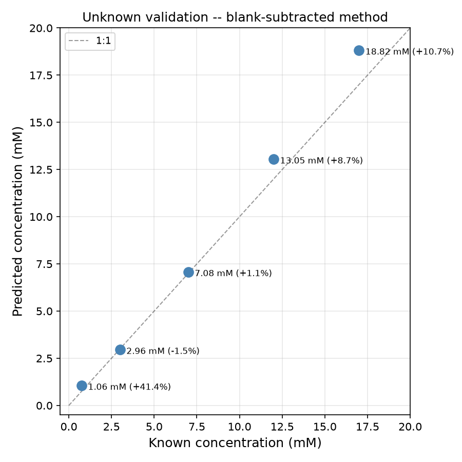
Figure 4. Predicted vs known concentration. Labels show predicted value and percent error.

Concentration	Known (mM)	dm (AU/um)	db (AU)	R2	Predicted (mM)	Error (mM)	Error (%)
0.75mM	0.75	0.000007	0.00001	0.98455	1.06	0.31	41.4
3mM	3.00	0.000060	0.00157	0.99035	2.96	-0.04	-1.5
7mM	7.00	0.000175	0.00572	0.99614	7.08	0.08	1.1
12mM	12.00	0.000342	0.00898	0.99551	13.05	1.05	8.7
17mM	17.00	0.000503	0.01214	0.99547	18.82	1.82	10.7

Table: Per-unknown prediction results with absolute and percent error.