Beer–Lambert law: $A = \varepsilon c \ell$
Because the same BPB solution fills all sections, $\varepsilon$ and $c$ are identical everywhere. The only variable is the optical path length $\ell$ — equal to the channel height $h$. Therefore the absorbance ratio between any two sections equals their height ratio:
$$\frac{A_i}{A_j} = \frac{h_i}{h_j}$$The 200 μm section (S1) was independently confirmed by focus-stepping to be exactly 200 μm. Using it as the calibration reference:
$$\hat{h}_i = 200\,\mu\text{m} \times \frac{A_i}{A_1}$$where $A_i = -\log_{10}(T_i)$ and $T_i$ is the dark-corrected transmittance in section $i$.
All raw intensities are dark-corrected before computing transmittance:
$$T_i = \frac{\langle I_\text{BPB} \rangle_i - \langle D \rangle_i} {\langle I_0 \rangle_i - \langle D \rangle_i}$$where $\langle \cdot \rangle_i$ denotes the spatial mean over ROI $i$, $I_\text{BPB}$ is the BPB sample image, $I_0$ is the pre-BPB light reference, and $D$ is the dark frame.
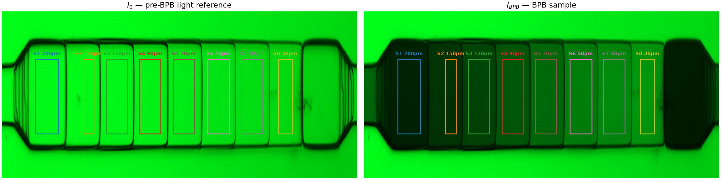
ROIs were adjusted interactively in the channel_heights.py marimo notebook
to align with the flat floors of each depth step in the BPB images, avoiding
the transition ramps. The row band (80–205 px) is shared with the flat-field
analysis notebook.
| Section | Depth | Col start | Col end | Width (px) |
|---|---|---|---|---|
| S1 | 200 µm | 160 | 270 | 110 |
| S2 | 150 µm | 390 | 440 | 50 |
| S3 | 120 µm | 500 | 600 | 100 |
| S4 | 90 µm | 660 | 760 | 100 |
| S5 | 70 µm | 820 | 920 | 100 |
| S6 | 50 µm | 985 | 1090 | 105 |
| S7 | 40 µm | 1145 | 1248 | 103 |
| S8 | 30 µm | 1322 | 1390 | 68 |
Left: pre-BPB light reference ($I_0$, 5 frames averaged). Right: BPB sample ($I_\text{BPB}$, 5 frames averaged). Deeper sections are visibly dimmer in the BPB image — more dye volume, greater absorption.
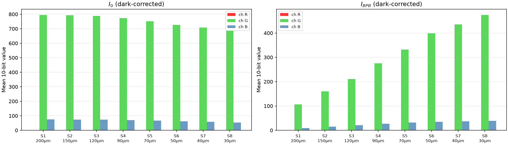
Per-section, per-channel means after subtracting the averaged dark frame. The G channel carries the dominant BPB absorption signal under the TRITC bandpass filter (~530–590 nm). The R channel is zero throughout (filter blocks all red-range wavelengths reaching the sensor).
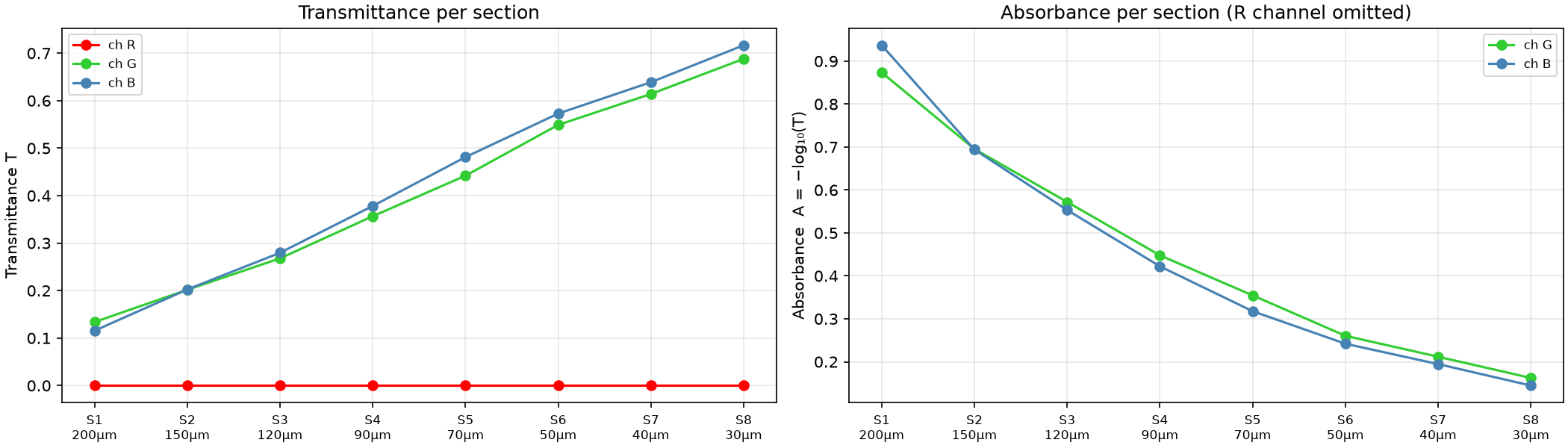
Transmittance: $T_i = \langle I_\text{BPB} \rangle_i \,/\, \langle I_0 \rangle_i$ (dark-corrected). Absorbance: $A_i = -\log_{10}(T_i)$.
The R channel is omitted from the absorbance plot — its signal is zero (fully blocked by the TRITC filter) so it contributes no useful information and obscures the G and B detail.
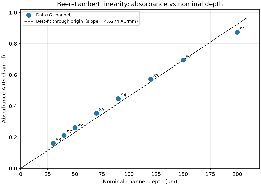
If Beer–Lambert holds, absorbance should be proportional to nominal depth and the data should fall on a line through the origin. The slope equals $\varepsilon c$ (absorptivity × concentration, in μm−1).
S1 (200 μm) lies slightly below the best-fit line through all eight points, while S3–S8 lie above. This pattern is consistent with stray light from the step-edge ramps reducing S1’s apparent absorbance (see Discussion).
Using the G-channel absorbance ratio relative to S1: $\hat{h}_i = 200\,\mu\text{m} \times A_i^G / A_1^G$
| Section | Nominal (µm) | Estimated (µm) | Deviation (µm) | Deviation (%) |
|---|---|---|---|---|
| S1 | 200 | 200.0 | +0.0 | +0.0% |
| S2 | 150 | 159.2 | +9.2 | +6.1% |
| S3 | 120 | 131.0 | +11.0 | +9.1% |
| S4 | 90 | 102.5 | +12.5 | +13.9% |
| S5 | 70 | 81.2 | +11.2 | +16.0% |
| S6 | 50 | 59.6 | +9.6 | +19.2% |
| S7 | 40 | 48.5 | +8.5 | +21.2% |
| S8 | 30 | 37.2 | +7.2 | +23.9% |
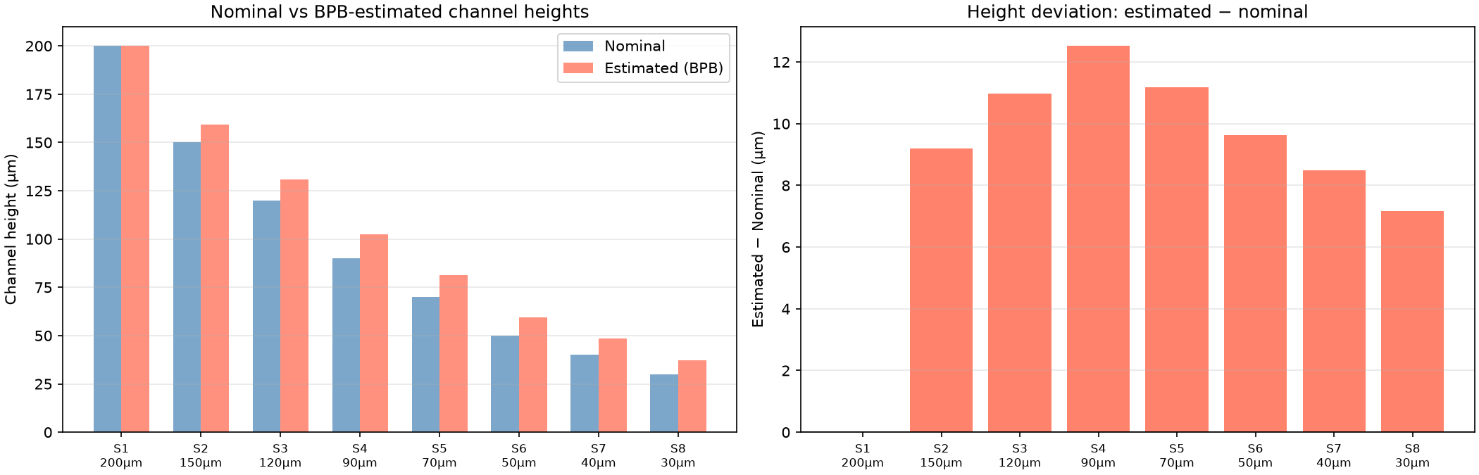
The ratio method yields only relative channel heights:
$$\hat{h}_i = h_\text{ref} \times \frac{A_i}{A_\text{ref}}$$The absolute scale is set entirely by the calibration reference — here $h_\text{ref} = 200\,\mu\text{m}$ from an independent focus-stepping measurement of S1. $\hat{h}_1 = 200\,\mu\text{m}$ is therefore trivially true by construction, not a result of the Beer–Lambert analysis. The method cannot detect any error in S1’s own height.
All sections S2–S8 are estimated as larger than their nominal design depths, with the discrepancy growing monotonically as sections get shallower:
| Section | Nominal (µm) | Estimated (µm) | Δ (µm) | Δ (%) |
|---|---|---|---|---|
| S1 | 200 | 200.0 | +0.0 | +0.0% |
| S2 | 150 | 159.2 | +9.2 | +6.1% |
| S3 | 120 | 131.0 | +11.0 | +9.1% |
| S4 | 90 | 102.5 | +12.5 | +13.9% |
| S5 | 70 | 81.2 | +11.2 | +16.0% |
| S6 | 50 | 59.6 | +9.6 | +19.2% |
| S7 | 40 | 48.5 | +8.5 | +21.2% |
| S8 | 30 | 37.2 | +7.2 | +23.9% |
A genuine uniform height excess of ~10 μm would produce a constant absolute deviation but a shrinking percentage deviation for deeper sections — the opposite of what is observed. The measured pattern (monotonically increasing percentage error for shallower sections) is the hallmark of stray light in the S1 ROI.
S1 is the deepest section, so BPB absorbs the most light there. The transmitted intensity $I_\text{BPB}$ in S1 is small — comparable to any scattered light $S$ leaking in from the bright step-edge ramps bordering the ROI. This inflates $T_1$ and reduces the measured $A_1$ below its true value:
$$T_{1,\text{apparent}} = \frac{I_{\text{BPB},1} + S}{I_{0,1} + S} > T_{1,\text{true}} \quad\Longrightarrow\quad A_{1,\text{apparent}} < A_{1,\text{true}}$$Using this underestimated $A_1$ as the calibration denominator inflates every ratio:
$$\hat{h}_i = 200 \times \frac{A_i}{A_{1,\text{apparent}}} > 200 \times \frac{A_i}{A_{1,\text{true}}} = h_i$$The effect is largest for the shallowest sections because their $A_i$ is approximately correct (little absorption → stray light is a small fraction of a large $I_\text{BPB}$), so the inflation comes almost entirely from the underestimated denominator. For the deeper sections (S2–S4) stray light also partially reduces their $A_i$, partially cancelling the effect and producing a smaller percentage overestimate than for S7–S8.