Characterise flat-field (light) drift across the full 2026-07-23 urea-assay experiment.
This dataset has a light-field capture after every concentration sample, giving 30 light images in total — far more temporal resolution than the 2026-07-16 dataset.
The channel is a DLP-3D-printed dense PEGDA network (Mn = 250 Da) imaged on an inverted Olympus IX71 (4× objective + 1.6× magnification, TRITC bandpass filter ~530–590 nm). Eight stepped-height sections (200 → 30 µm) span the field of view.
process.txt)| Phase | Light captures | Clock range |
|---|---|---|
| Initial | initial/initial light |
15:43 |
| Sample set 1 (13 conc., ascending) | post-sample light after each | 15:54 – 16:31 |
| Between sets | between/light |
16:41 |
| Sample set 2 (13 conc., ascending) | post-sample light after each | 16:44 – 17:17 |
| Bromophenol blue | pre + post BPB light | 17:19 – 17:22 |
Each post-sample light is taken after the sample is run and the channel is flushed with blank buffer. The between-sets light follows a fresh buffer flush between the two sample runs.
Questions addressed:
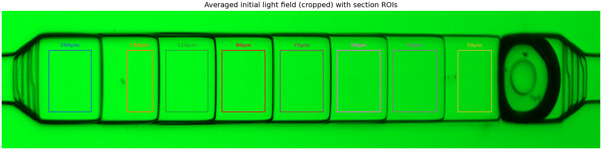
crop_and_roi.py)All coordinates in cropped-image space. Row band 80–205 px shared across all sections. Each column extent covers the flat interior of that depth step, avoiding the transition ramps.
| Section | Depth | Cropped columns |
|---|---|---|
| S1 | 200 µm | 133–253 |
| S2 | 150 µm | 355–427 |
| S3 | 120 µm | 465–585 |
| S4 | 90 µm | 625–747 |
| S5 | 70 µm | 790–912 |
| S6 | 50 µm | 952–1074 |
| S7 | 40 µm | 1110–1235 |
| S8 | 30 µm | 1295–1390 |
The image below is the averaged initial light field (30 frames, in cropped coordinates). Coloured boxes mark the 8 section ROIs used for all quantitative analysis; labels give the depth of each step. Note that deeper sections appear brighter — a genuine optical property of the channel geometry under transmitted illumination, and the reason a per-sample flat-field correction is essential.
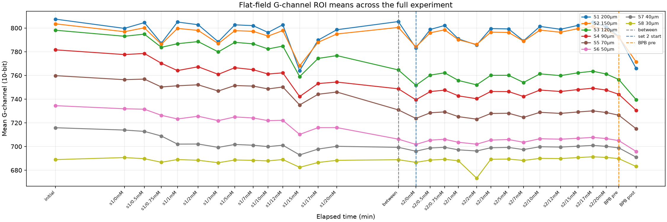
Each line is one stepped-height section; points are the per-capture mean G-channel value. Vertical dashed lines mark phase boundaries: grey = between sets, blue = set 2 start, orange = BPB pre-light.
Deeper sections appear brighter throughout because the longer optical path through more PEGDA material transmits more illumination in this spectral range — a genuine optical property of the channel geometry, not noise.
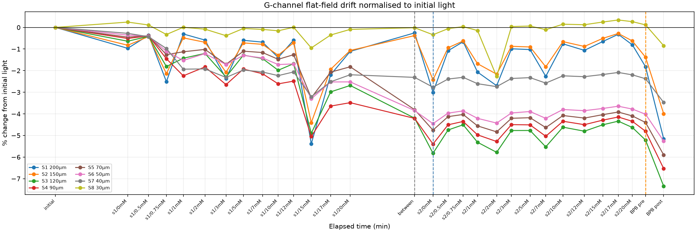
Values expressed as % change from the initial/initial light baseline, making it easier
to compare the magnitude and direction of drift across sections.
Key observations: - Drift is non-monotonic: values bounce by a few percent across the 30 captures but do not follow a single consistent upward or downward trend. - The shallowest section (S8, 30 µm) stays within ±0.5% — almost negligible. - The deepest section (S1, 200 µm) drifts more (±1–5%) but non-monotonically. - The intermediate sections (S3–S6, 120–50 µm) show the largest variability (1–2% std).
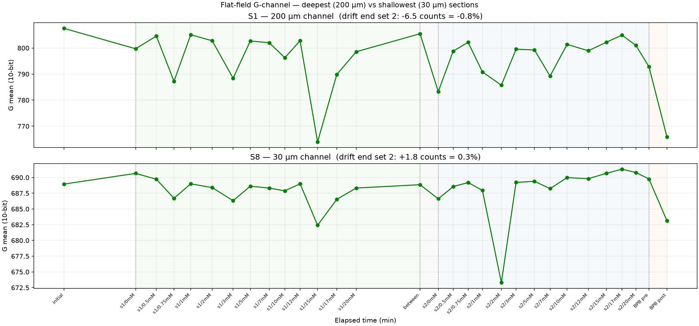
These two extreme sections bracket the range of behaviour. Phase bands show which part of the experiment each capture belongs to (light green = set 1, light blue = set 2, light orange = BPB).
S8 (30 µm) is remarkably stable — its flat-field is essentially constant across the entire experiment. S1 (200 µm) shows low-frequency non-monotonic excursions, likely driven by small focus or position drifts that shift how much scattered light from the step-edge ramps falls into the 200 µm ROI.
Bar chart showing the % change from initial at four checkpoints. There is no consistent monotonic depth-dependence across sections: unlike the 2026-07-16 dataset (which showed a clear depth gradient from BTB residue), the 2026-07-23 drift is dominated by non-monotonic, section-specific fluctuations.
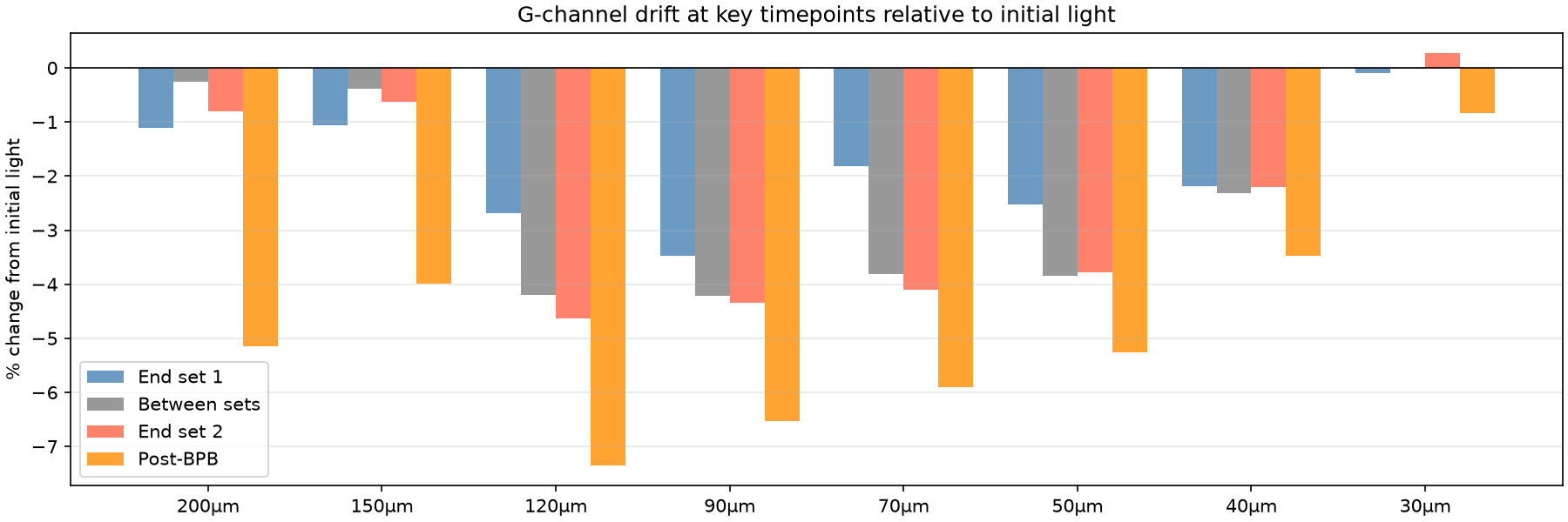
| Timepoint | Phase | S1 200µm G | S1 % from init | S8 30µm G | S8 % from init |
|---|---|---|---|---|---|
| initial | initial | 807.5 | +0.0% | 689.0 | +0.0% |
| s1/0mM | set1 | 799.7 | -1.0% | 690.7 | +0.2% |
| s1/0.5mM | set1 | 804.6 | -0.4% | 689.7 | +0.1% |
| s1/0.75mM | set1 | 787.2 | -2.5% | 686.7 | -0.3% |
| s1/1mM | set1 | 805.1 | -0.3% | 689.0 | +0.0% |
| s1/2mM | set1 | 802.8 | -0.6% | 688.4 | -0.1% |
| s1/3mM | set1 | 788.4 | -2.4% | 686.3 | -0.4% |
| s1/5mM | set1 | 802.7 | -0.6% | 688.6 | -0.0% |
| s1/7mM | set1 | 802.0 | -0.7% | 688.3 | -0.1% |
| s1/10mM | set1 | 796.3 | -1.4% | 687.9 | -0.2% |
| s1/12mM | set1 | 802.8 | -0.6% | 689.0 | +0.0% |
| s1/15mM | set1 | 764.0 | -5.4% | 682.4 | -0.9% |
| s1/17mM | set1 | 789.8 | -2.2% | 686.5 | -0.4% |
| s1/20mM | set1 | 798.6 | -1.1% | 688.3 | -0.1% |
| between | between | 805.5 | -0.3% | 688.9 | -0.0% |
| s2/0mM | set2 | 783.2 | -3.0% | 686.6 | -0.3% |
| s2/0.5mM | set2 | 798.8 | -1.1% | 688.6 | -0.1% |
| s2/0.75mM | set2 | 802.2 | -0.7% | 689.2 | +0.0% |
| s2/1mM | set2 | 790.8 | -2.1% | 688.0 | -0.1% |
| s2/2mM | set2 | 785.7 | -2.7% | 673.3 | -2.3% |
| s2/3mM | set2 | 799.5 | -1.0% | 689.2 | +0.0% |
| s2/5mM | set2 | 799.2 | -1.0% | 689.4 | +0.1% |
| s2/7mM | set2 | 789.2 | -2.3% | 688.2 | -0.1% |
| s2/10mM | set2 | 801.4 | -0.8% | 690.0 | +0.1% |
| s2/12mM | set2 | 798.9 | -1.1% | 689.8 | +0.1% |
| s2/15mM | set2 | 802.2 | -0.7% | 690.7 | +0.2% |
| s2/17mM | set2 | 804.9 | -0.3% | 691.3 | +0.3% |
| s2/20mM | set2 | 801.0 | -0.8% | 690.8 | +0.3% |
| BPB pre | bpb | 792.8 | -1.8% | 689.8 | +0.1% |
| BPB post | bpb | 765.9 | -5.2% | 683.1 | -0.8% |
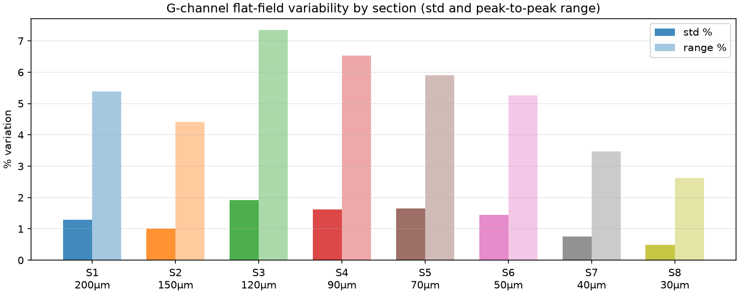
Variability is expressed as the standard deviation and peak-to-peak range of the G-channel % drift (relative to initial light) across all 30 light captures.
The intermediate sections (S3–S6, 120–50 µm) show the largest spread — both in std and peak-to-peak range. The shallowest section (S8, 30 µm) is the most stable.
What is the Pearson correlation coefficient (r)? The Pearson r measures how closely two quantities rise and fall together across a set of measurements. It ranges from −1 to +1:
| r value | Meaning |
|---|---|
| +1.00 | Perfect positive correlation — when one goes up, the other always goes up by a proportional amount |
| ~0.9–1.0 | Strong positive correlation |
| ~0.5–0.9 | Moderate positive correlation |
| ~0 | No linear relationship — the two quantities change independently |
| Negative | When one goes up, the other tends to go down |
Here, each pair of sections has its % drift values (one per light capture, 30 values total) compared. An r near +1 means those two sections experience nearly identical flat-field fluctuations; an r near 0 means their fluctuations are unrelated.
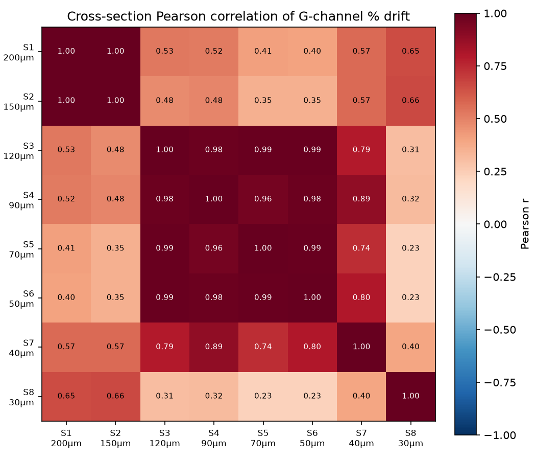
The 8 sections fall into distinct correlation groups:
| Group | Sections | Internal r | Between-group r |
|---|---|---|---|
| Deep | S1 (200 µm), S2 (150 µm) | ~1.00 | 0.35–0.53 |
| Intermediate | S3–S6 (120–50 µm) | 0.96–0.99 | 0.23–0.53 |
| Shallow | S8 (30 µm) | — | 0.23–0.66 |
| Transitional | S7 (40 µm) | — | 0.40–0.89 |
Sections within a group rise and fall together almost perfectly; sections across groups are nearly uncorrelated. This rules out a single global cause (illumination lamp flicker would move all sections in unison, giving r ≈ 1 everywhere).
The step transition ramps between adjacent sections scatter and redirect light laterally. The intermediate sections (50–120 µm) are flanked on both sides by sections of different depth, so they receive stray light contributions from two ramps. The deepest (200 µm) and shallowest (30 µm) sections are at the edges of the channel geometry and have fewer competing ramps, making them less susceptible to cross-talk from step-edge scatter. Small shifts in device position or focus — sub-micron motions from syringe pumping or wicking — would change how much scattered light falls in the intermediate ROIs without appreciably shifting the edge sections, producing the observed group-correlated but cross-group-uncorrelated fluctuations.
| Metric | Value | Comment |
|---|---|---|
| S8 (30 µm) std | 0.49 % | Negligible; well below assay signal |
| S1 (200 µm) std | 1.29 % | Acceptable; within-group fluctuations shared |
| S3–S6 (120–50 µm) std | 1.4–1.9 % | Largest variability; limits flat-field accuracy |
| Within-burst shot noise | ~0.02 % | Not the limiting factor |
The per-sample post-sample light design is the correct mitigation: each sample's transmittance is normalised by the flat-field immediately after the buffer flush for that sample, so slow drift is fully corrected. What remains uncorrected is any flat-field change that occurs between the sample image acquisition and the subsequent post-sample light capture — essentially the ~2–3 minute window of sample flow and flushing.
For low urea concentrations (≤1 mM) where the phenol red absorbance change is small, the 1–2% residual uncertainty in the intermediate sections is the dominant systematic error. The 200 µm and 30 µm sections, being the least affected, may give the cleanest low-concentration signal. At high concentrations (≥5 mM) where the signal is large, even a 2% flat-field uncertainty is unimportant.