Allura Red Dye with 510/10 Narrow-Bandpass Filter

Purpose

This notebook designs the absorption-based measurement approach for a microfluidic stepped-height observation channel experiment. The device presents eight nominal channel heights (30, 40, 50, 70, 90, 120, 150, and 200 µm), all filled with the same Allura Red dye solution at a single working concentration. Channel height at each step is inferred from the measured polychromatic absorbance $A_\text{meas}$.

Three questions drive the analysis:

1. Dye–filter compatibility — does Allura Red's absorption peak overlap the 510/10 nm narrow-bandpass filter sufficiently, and is the polychromatic Beer-Lambert error small enough to treat $A_\text{meas}$ as linear in height?

2. Working concentration — what Allura Red concentration places $A_\text{meas}$ in a useful measurement window (0.05–0.80 AU) across all eight step heights?

3. Calibration strategy — how do we infer height from $A_\text{meas}$ without depending on tabulated molar absorptivity values or precisely known stock concentrations? The chosen approach uses an 80 µm microscope-slide capillary filled with Allura Red solutions at known dilutions to generate an empirical $A_\text{meas}$ vs. effective path-length curve.

The analysis proceeds in order through these three questions, finishing with a practical recommendation for a four-concentration capillary calibration set.

Spectral overview: Allura Red × 510/10 compatibility

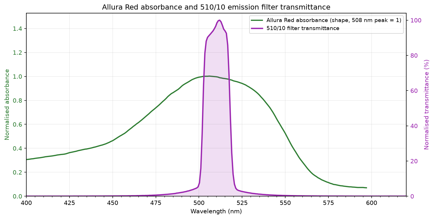
Allura Red (FD&C Red 40) has a visible absorption peak near 506 nm with a molar absorptivity $\varepsilon_{508} \approx 2.59\times10^4$ L mol$^{-1}$ cm$^{-1}$. The 510/10 nm narrow-bandpass filter (nominally 5 nm half-bandwidth, centred at 510 nm) sits directly on this peak, maximising signal and minimising the polychromatic Beer-Lambert error that arises when the filter passband spans a region of varying absorbance.

The plot below overlays the normalised Allura Red absorbance (left axis) and the measured 510/10 filter transmittance (right axis). The digitized absorbance spectrum was obtained from the Allura Red AC absorption spectrum.

Concentration selection

The stepped-height channel has eight nominal observation heights spanning a 6.7× range (30–200 µm). Because Beer-Lambert absorbance is proportional to the product $C \cdot L$, a single dye concentration must produce a measurable signal at the shallowest step and remain in a linear regime at the deepest.

The target absorbance window is 0.05–0.80 AU: the lower bound keeps shallow channels above the noise floor; the upper bound stays below the region where detector nonlinearity and stray light introduce significant error.

Polychromatic absorbance is computed by integrating Beer-Lambert over the filter passband:

$$A_\text{meas} = -\log_{10}\!\left(\frac{\int F(\lambda)\,10^{-A(\lambda)}\,d\lambda}{\int F(\lambda)\,d\lambda}\right), \quad A(\lambda) = \varepsilon(\lambda)\,C\,L$$

The sweep below evaluates $A_\text{meas}$ for eight concentrations across all channel heights to identify the working concentration.

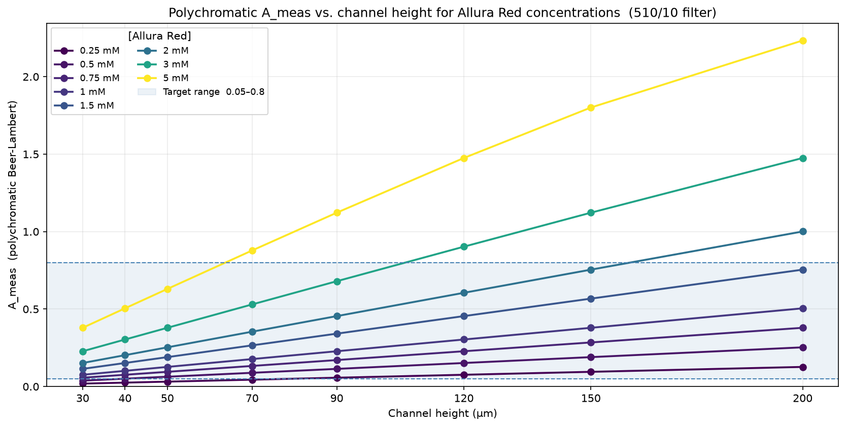
Chosen working concentration: 1.0 mM Allura Red.

At 1.0 mM the polychromatic $A_\text{meas}$ spans 0.076 (30 µm) to 0.505 (200 µm) — all eight step heights land comfortably within the target measurement range of 0.05–0.80.

Capillary calibration concentrations

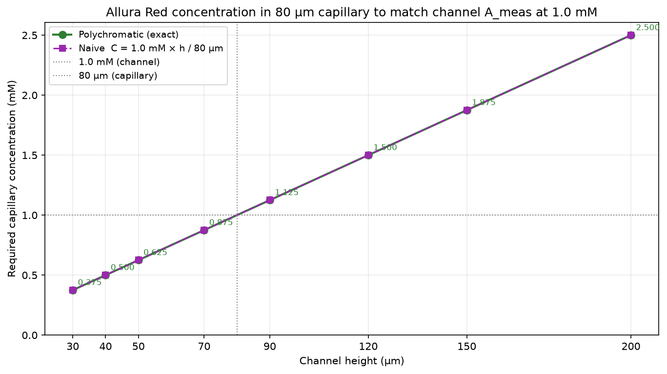
To use an 80 µm microscope slide capillary gap as a calibration standard, we need to identify the Allura Red concentration $C_\text{cal}$ that produces the same polychromatic $A_\text{meas}$ as each channel step height filled with 1.0 mM dye.

From Beer-Lambert, the naive estimate is simply

$$C_\text{cal}(h) = 1.0\,\text{mM} \times \frac{h}{80\,\mu\text{m}}$$

Because the polychromatic error for Allura Red × 510/10 is very small (< 0.5 %), the naive formula is highly accurate, but we compute the exact polychromatic-corrected value by numerically inverting $A_\text{meas}(80\,\mu\text{m},\, C_\text{cal}) = A_\text{target}(h)$ over a dense concentration grid.

Capillary calibration concentrations — Allura Red × 510/10 filter

Does the capillary calibration provide a benefit?

Yes — primarily by removing two sources of systematic error and implicitly correcting for real measurement-system effects.

Image correction

Every image in this experiment will be fully corrected before computing absorbance:

$$I = \frac{I_\text{sample} - I_\text{dark}}{I_0 - I_\text{dark}}$$

where $I_\text{dark}$ is a dark-field image (sensor noise with no light) and $I_0$ is a flat-field blank image taken with pure solvent in the capillary or channel. This correction removes dark current, spatial non-uniformity in the illumination, and pixel-to-pixel sensitivity variation. Absorbance is then $A = -\log_{10} I$.

Because both the capillary calibration images and the stepped-channel images receive the same correction procedure, flat-field and dark-field errors cancel in both cases.

Remaining error sources — where capillary calibration helps

1. Molar absorptivity uncertainty. The value $\varepsilon_{508} = 2.59\times10^4$ L mol$^{-1}$ cm$^{-1}$ was estimated from a digitized literature plot. The true value for this dye batch, solvent, pH, and temperature could differ by several percent. A direct Beer-Lambert height calculation propagates that uncertainty straight into $h$. Capillary calibration eliminates $\varepsilon$ entirely: the empirical $A_\text{meas}$ vs. $C \cdot L$ curve is measured rather than predicted, so no absorptivity value is needed.

2. Absolute stock concentration uncertainty. If the nominal 1.0 mM stock is actually 0.97 mM, every inferred height is off by 3%. Preparing the calibration dilutions from the same stock as the channel fill — $C_\text{cal} = C_\text{stock} \times h/80\,\mu\text{m}$ — means the absolute stock concentration cancels in the height ratio:

$$h = 80\,\mu\text{m} \times \frac{C_\text{cal}}{C_\text{channel}}$$

regardless of what $C_\text{stock}$ actually is. Only the relative dilution accuracy matters.

3. Residual detector and system effects. Any deviation of the real optical system from ideal Beer-Lambert behavior (residual stray light, camera nonlinearity, the actual vs. nominal filter transmission profile) affects capillary and channel measurements identically, so it cancels when heights are inferred from the empirical calibration curve rather than from a theoretical prediction.

Why this works cleanly for Allura Red × 510/10

The polychromatic Beer-Lambert error for this dye–filter combination is less than 0.5 % across the full concentration and height range of interest. This means the $A_\text{meas}$ vs. $C \cdot L$ relationship is essentially linear and well-behaved, making the capillary calibration curve smooth and directly invertible.

Practical conclusion

Use the capillary calibration as the primary height inference method. Direct Beer-Lambert prediction (using $\varepsilon_{508}$ and nominal concentration) serves as a cross-check. If the two agree, confidence in the inferred heights is high. If they disagree, the capillary result is more trustworthy because it is independent of $\varepsilon$ and absolute concentration.

Height resolution: detecting 3–10 µm deviations from nominal

Absorbance sensitivity to height

Because the polychromatic error for Allura Red × 510/10 is less than 0.5 %, $A_\text{meas}$ is essentially linear in height:

$$\frac{dA}{dh} = \varepsilon_\text{eff} \cdot C = 2.59\times10^4\,\frac{\text{L}}{\text{mol}\cdot\text{cm}} \times 1.0\times10^{-3}\,\frac{\text{mol}}{\text{L}} \times 10^{-4}\,\frac{\text{cm}}{\mu\text{m}} \approx 2.59\times10^{-3}\;\text{AU}/\mu\text{m}$$

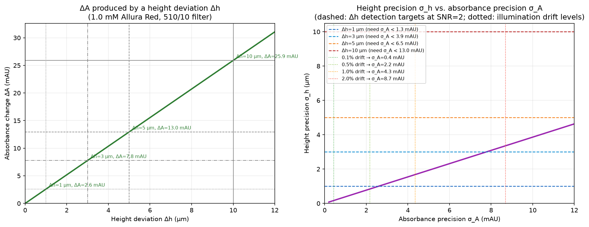
Crucially, $\Delta A = (dA/dh)\,\Delta h$ is constant — independent of the nominal channel height. The height resolution is therefore:

$$\sigma_h = \frac{\sigma_A}{dA/dh} \approx 386\,\mu\text{m} \times \sigma_A$$

Practical limits on $\sigma_A$

With flat-field and dark-field correction applied, photon shot noise is negligible once a modest number of pixels are averaged. The dominant error source is illumination drift between the $I_0$ (blank) and $I_\text{sample}$ acquisitions. A fractional drift $\delta$ in lamp intensity appears as a systematic $\sigma_A \approx \delta/\ln 10$.

Taking $I_0$ with a fully warmed-up lamp and bracketing it tightly around the sample acquisition should keep drift below 0.5 %, giving $\sigma_h < 1\,\mu\text{m}$.

Detectability of $\Delta h$ deviations

A deviation $\Delta h$ is reliably detected when $\Delta A > 2\sigma_A$ (SNR > 2). The plots below show $\Delta A$ for target deviations and the $\sigma_A$ required to detect them at SNR ≥ 2.

Single-reference vs. multi-concentration capillary calibration

Strategy A — concentration series matched to each nominal height

Prepare eight solutions at $C_\text{cal}(h) = 1.0\,\text{mM} \times h/80\,\mu\text{m}$ and measure each in the 80 µm capillary. Each measurement reproduces the Beer-Lambert product $C \cdot L$ for the corresponding channel step, giving an empirical $(A_\text{meas},\, h_\text{equiv})$ calibration curve.

Strategy B — single reference at 1.0 mM

Fill the capillary once with 1.0 mM dye and measure $A_\text{cal}$. Infer channel heights from the ratio:

$$h = 80\,\mu\text{m} \times \frac{A_\text{channel}}{A_\text{cal}}$$

What Strategy B still eliminates

The ratio form means $\varepsilon$ and the absolute stock concentration both cancel — any proportional error in $C$ shifts $A_\text{channel}$ and $A_\text{cal}$ by the same factor, leaving $h$ unchanged. Strategy B therefore provides the same immunity to $\varepsilon$ uncertainty and concentration uncertainty as the full series.

The real downside of Strategy B: no linearity check

Strategy B commits to a perfectly linear $A_\text{meas}$ vs. $h$ relationship through a single point at $A \approx 0.203$ AU (80 µm, 1.0 mM). If the camera has a small nonlinearity, or if stray light reaches the detector, heights at the shallow (30–50 µm, $A \approx 0.076$–$0.127$ AU) and deep (150–200 µm, $A \approx 0.379$–$0.505$ AU) extremes carry a systematic error that cannot be detected or corrected from a single calibration point. The 8-concentration series would immediately reveal any deviation from linearity as curvature in the $A_\text{meas}$ vs. $C \cdot L$ plot.

Two smaller concerns

Calibration noise propagation. A single $A_\text{cal}$ measurement carries its full uncertainty into every height estimate. With a multi-point series you can average or fit, reducing the calibration noise floor. This matters most for shallow heights ($h \approx 30$–50 µm), where $A_\text{channel} \approx A_\text{cal}/3$ so errors in $A_\text{cal}$ are amplified by the same factor.

Extrapolation in both directions. The single reference sits at $A \approx 0.203$ AU. Shallow heights require extrapolating downward to $A \approx 0.076$ AU; deep heights require extrapolating upward to $A \approx 0.505$ AU. The series brackets the full range.

Practical recommendation

For a well-characterised 16-bit camera in this intensity range ($I/I_0 \approx 0.31$–$0.84$), detector nonlinearity is typically well below 0.5 % — comparable to or smaller than the illumination-drift budget. Strategy B is likely adequate for a first experiment.

A pragmatic middle ground: use 1.0 mM as the primary reference, but also measure at one or two additional concentrations (e.g. 0.375 mM and 1.875 mM, the equivalents of 30 µm and 150 µm) to verify linearity without preparing all eight solutions. If those three points are collinear, Strategy B is validated. If they are not, the deviation is caught early and the full series can be prepared for a follow-up experiment.

A practical four-concentration calibration set

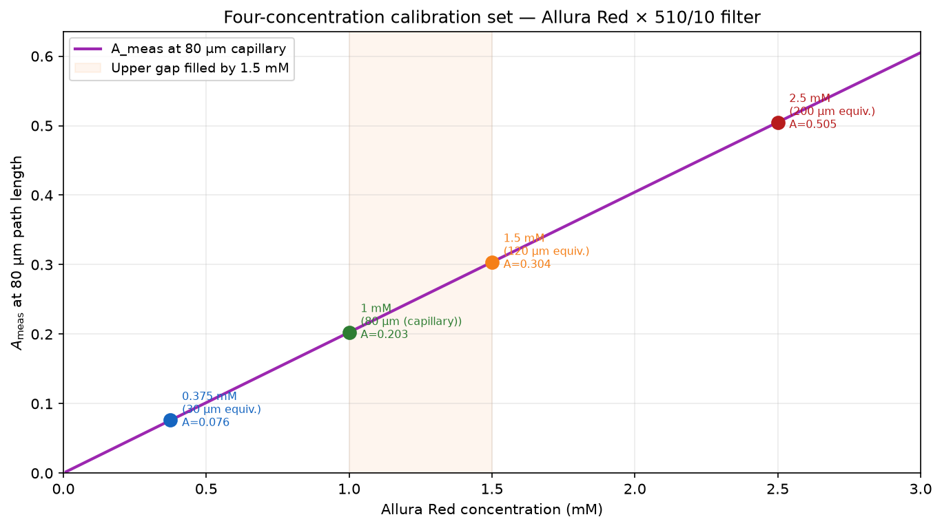
The analysis above identifies two extremes: a single 1.0 mM reference (fast but no linearity check) and a full eight-concentration series (complete but time-consuming to prepare). A useful middle ground is four concentrations that bracket the full measurement range and provide a meaningful linearity test.

Chosen concentrations

Why 1.5 mM as the fourth point?

The three "required" points — 0.375, 1.0, and 2.5 mM — cover the full absorbance range but with uneven spacing. The gap between 1.0 and 2.5 mM ($\Delta A = 0.302$ AU) is more than twice the gap between 0.375 and 1.0 mM ($\Delta A = 0.127$ AU). Adding 1.5 mM at $A \approx 0.304$ AU fills the upper gap and produces a nearly uniform distribution:

$$0.076 \to 0.203 \to \mathbf{0.304} \to 0.505$$

The upper portion of the curve ($A > 0.2$ AU) is also where detector saturation effects and stray light are most likely to cause nonlinearity, so this is where the extra coverage matters most.

Linearity-checking power

With four points along a nominally linear relationship, a linear fit uses two parameters and leaves two residuals — enough to detect systematic curvature that would be invisible with only three points (one residual). If all four points fall on a straight line within measurement noise, Strategy B (single 1.0 mM reference) is validated. If they do not, the deviation is quantified and a corrected polynomial fit can be used instead.

Preparation from a single 2.5 mM stock

Multiple concentrations in the stepped-height channel

Running the channel at a second Allura Red concentration adds five distinct capabilities that the capillary calibration alone cannot provide.

1. Internal Beer–Lambert linearity test at every height

At each height step $h_i$, two concentrations give two measurements governed by the same physics:

$$A(h_i,\, C_1) = \varepsilon_\text{eff}\cdot C_1\cdot h_i \qquad\qquad A(h_i,\, C_2) = \varepsilon_\text{eff}\cdot C_2\cdot h_i$$

Their ratio eliminates every unknown except the concentration ratio you control:

$$\frac{A(h_i,\, C_2)}{A(h_i,\, C_1)} = \frac{C_2}{C_1}$$

This ratio is independent of $h_i$, $\varepsilon_\text{eff}$, and the capillary calibration — a direct test of Beer–Lambert linearity at the actual channel absorbances, not at the 80 µm capillary path length. Any deviation from $C_2/C_1$ indicates detector nonlinearity or stray light at the relevant absorbance values.

2. Relative step heights with zero calibration

At fixed concentration, the ratio of absorbances across two heights gives the height ratio directly:

$$\frac{A(h_1,\, C_j)}{A(h_2,\, C_j)} = \frac{h_1}{h_2}$$

No $\varepsilon$, no stock concentration, no capillary measurement. Designed step ratios (e.g. 40 µm / 30 µm = 1.33, 200 µm / 100 µm = 2.00) can be verified purely from the channel images.

3. Decouple height from $\varepsilon \cdot C$

With a single concentration, $h$ and $\varepsilon \cdot C$ appear only as a product and cannot be separated. With two concentrations whose ratio $C_2/C_1$ is accurately known, there are two equations and two unknowns ($h$ and $\varepsilon \cdot C_1$). Fitting a line through the origin to the points $(C_j,\, A(h_i, C_j))$ gives slope $\varepsilon \cdot h_i$ for each step — relative heights without any external calibration.

4. Catches geometry-dependent systematic errors

The capillary (80 µm slide gap) and the etched channel differ in surface character, meniscus geometry, and lateral uniformity. The capillary calibration tests the optical system at 80 µm but cannot detect a systematic offset between the two geometries. Multiple channel concentrations reveal any such offset as a concentration-independent bias in the $A$ vs. $C$ relationship — visible only when the measurement is repeated at a different concentration.

5. Redundant estimates improve precision

With $n$ concentrations, each height step yields $n$ independent estimates of $h$. A least-squares fit through the origin reduces height uncertainty by $1/\sqrt{n}$ and makes systematic curvature visible as a trend in the fit residuals, distinct from random measurement scatter.

Practical implementation: 1.0 mM + 1.5 mM

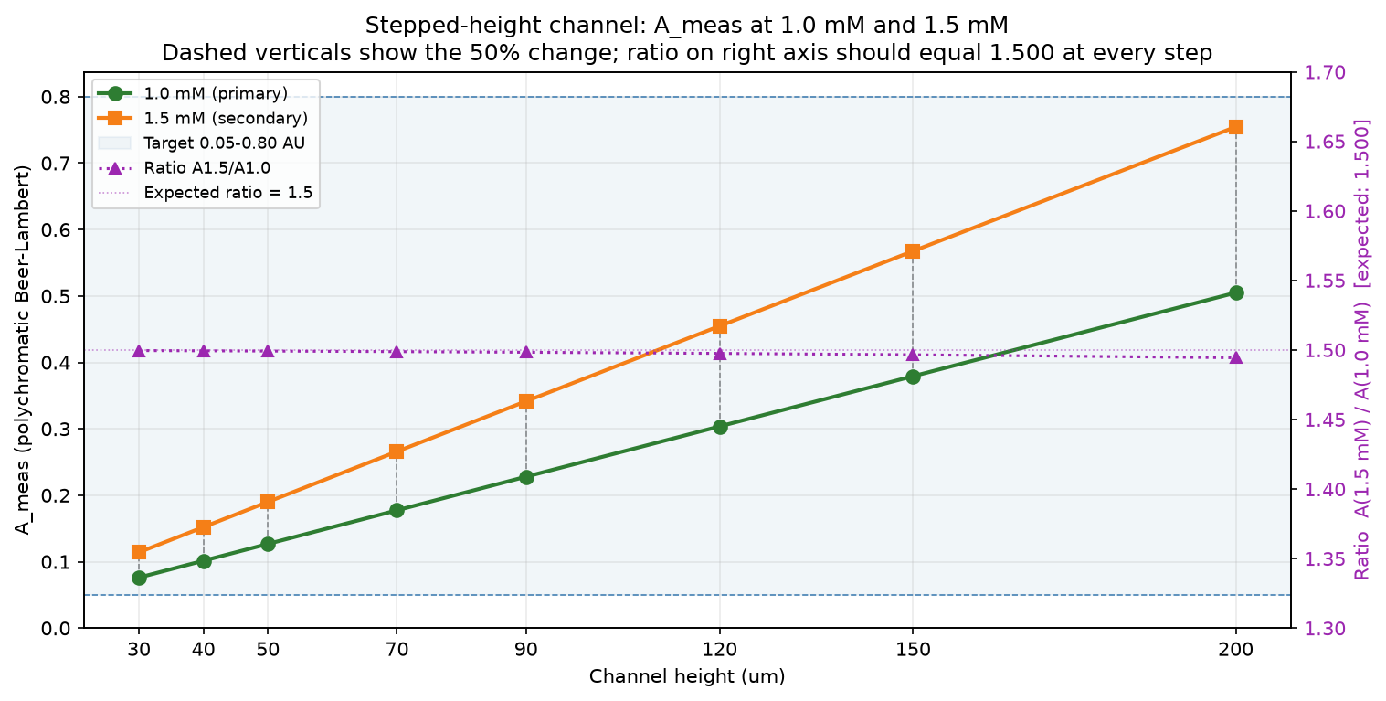
The secondary concentration should provide a large enough change to detect nonlinearity confidently while keeping all heights within the 0.05–0.80 AU measurement window. At 1.5 mM every step remains in-window, and the 50% concentration change produces a 50% change in $A_\text{meas}$. If the system is linear, the ratio $A_{1.5}/A_{1.0}$ equals exactly 1.500 at every step; deviations identify where the system departs from ideal Beer–Lambert behavior.

Conveniently, 1.5 mM is already in the four-concentration capillary calibration set, so no additional solution preparation is needed.

A_meas at 1.0 mM and 1.5 mM in each channel section (polychromatic Beer–Lambert model)

Single capillary concentration: accuracy and limitations

Using one capillary fill — 1.0 mM in the 80 µm gap, same stock as the channel — gives the height estimate:

$$h_i = 80\,\mu\text{m} \times \frac{A_\text{ch}(h_i)}{A_\text{cal}}$$

Both $\varepsilon_\text{eff}$ and the absolute stock concentration cancel exactly in this ratio. Flat-field and dark-field corrections apply identically to both acquisitions. Random photometric noise on $A_\text{cal}$ can be reduced by averaging many camera frames, so a single capillary fill is not fundamentally limited by calibration noise.

What is lost: the ability to detect nonlinearity

With one capillary point at $A_\text{cal} \approx 0.203$ AU there is no way to know whether the detector response is truly linear across the full absorbance range the channel spans (0.076–0.505 AU). Any nonlinearity — from camera response or stray light — creates a height-dependent systematic bias that is anchored to zero at $h = 80\,\mu\text{m}$ and grows toward the shallow and deep extremes.

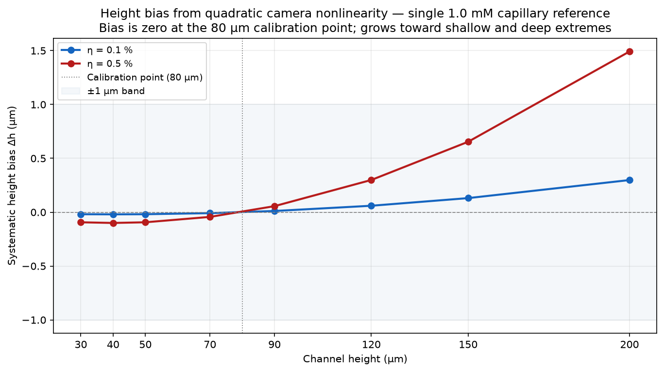
For a quadratic camera nonlinearity of fractional amplitude $\eta$ (the fractional deviation from linearity at the calibration absorbance $A_\text{cal}$), the height bias is:

$$\Delta h_i = h_i \cdot \eta \cdot \frac{A_i - A_\text{cal}}{A_\text{cal}}$$

This is zero at the calibration height (80 µm), negative for shallow steps ($A_i < A_\text{cal}$), and positive for deep steps ($A_i > A_\text{cal}$).

The distinguishability problem

With a single capillary concentration you cannot distinguish between:

• The 200 µm step is actually 201.5 µm — a real fabrication deviation, and
• The 200 µm step is exactly 200 µm but detector nonlinearity makes it read as 201.5 µm.

With two or more capillary concentrations the ratio $A_{C_2}/A_{C_1}$ at the capillary path length directly tests linearity. If the ratio holds, any observed height deviation is real.

Practical bottom line

For a well-characterised 16-bit scientific camera ($\eta < 0.2\,\%$), the systematic bias is well below 0.5 µm across the full height range — smaller than the illumination-drift budget. A single capillary concentration is a reasonable first experiment. The limitation matters when you need to trust individual height deviations at the 1–3 µm level: at that point a two-concentration capillary check is worth the extra solution preparation.

Systematic height bias Δh from quadratic camera nonlinearity (η = 0.1 % and 0.5 %) using a single 1.0 mM capillary reference at 80 µm

All four calibration concentrations in the stepped-height channel

If the four concentrations prepared for the capillary calibration (0.375, 1.0, 1.5, and 2.5 mM) are also run through the stepped-height channel, the out-of-range combinations at the extremes still deliver real analytical value.

Coverage

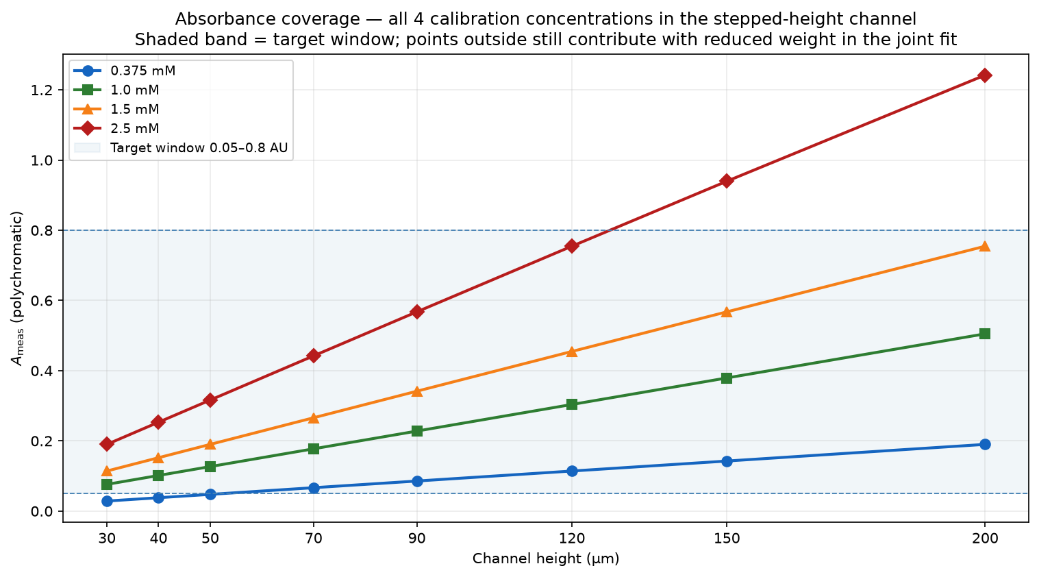
Not every combination of height and concentration lands in the target window. At 0.375 mM the shallowest steps (30–40 µm) produce $A < 0.05$; at 2.5 mM the deepest steps (150–200 µm) exceed $A = 0.80$. The middle two concentrations (1.0 and 1.5 mM) fall in range at all eight heights. The coverage matrix below shows the computed $A_\text{meas}$ values.

Out-of-range ≠ useless

"Out of range" means reduced precision, not invalid data. The polychromatic Beer–Lambert model is valid at all absorbances; the target window defines where signal-to-noise is best, not where the model breaks down. Out-of-range measurements enter a weighted fit with weight $w \propto 1/\sigma_A^2$, naturally suppressing their influence while preserving their contribution to the global solution.

The key gain: jointly fitting $\eta$ from the channel data

With a single channel concentration, the camera nonlinearity parameter $\eta$ must be imported from a separately calibrated capillary measurement. With multiple concentrations spanning a wide dynamic range, $\eta$ becomes a parameter the channel data can determine on its own.

The argument is geometric: for a fixed height $h$, a quadratic nonlinearity shifts the absorbance at 2.5 mM much more (in absolute AU) than at 0.375 mM. That differential shift is a unique signature of $\eta$ — it cannot be mimicked by a change in $h$ alone. Formally, the fit is cast as:

$$\min_{\{h_i\},\,\eta} \sum_{i,k} w_{ik}\bigl[A_\text{meas}(h_i, C_k) - A_\text{theory}(h_i, C_k, \eta)\bigr]^2$$

where the index $k$ runs over the four concentrations. The degrees of freedom for the joint fit (using $N_s = 8$ height sections) are:

With 23 degrees of freedom and a concentration span of 6.7× (0.375 to 2.5 mM), $\eta$ is tightly determined from the channel measurements alone. The capillary measurements — themselves at all four concentrations — then serve as consistency anchors on the absolute concentration scale rather than the sole source of systematic-error correction.

A_meas at all 4 concentrations × all 8 channel heights (✓ within 0.05–0.80 AU, ≈ marginal, ✗ outside)

Do the capillary measurements add anything?

With four concentrations in the stepped-height channel, the joint fit for $\{h_i\}$ and $\eta$ is strongly overdetermined (+23 DoF). A natural question is whether the capillary measurements are still needed at all.

The channel fit is nearly self-sufficient — with one caveat

The channel data fully determines:

• All height ratios $h_i / h_j$ — pinned by the shape of the $A_\text{meas}$ vs.\ $C$ curve, which is unique to each height
• The nonlinearity parameter $\eta$ — determined by the differential absorbance shift across the 6.7× concentration span

What it cannot determine on its own is the absolute height scale.

The scale degeneracy — and it is exact

Beer–Lambert absorbance depends only on the product $C \cdot h$. Therefore:

$$A_\text{theory}\!\bigl(h_i,\; C_k(1+\delta)\bigr) \;=\; A_\text{theory}\!\bigl(h_i(1+\delta),\; C_k\bigr)$$

This equality is exact, not approximate. A uniform $(1+\delta)$ factor on all concentrations is a perfect alias for the same factor on all heights — the two scenarios produce identical $A_\text{meas}$ values at every (height, concentration) pair. The compute cell below confirms $|\Delta A| = 0$ numerically.

The fit cannot distinguish "all concentrations were 2% high" from "all heights are 2% larger." It returns correct ratios $h_i/h_j$ and correct $\eta$, but all absolute values shift by $(1+\delta)$.

What the capillary measurements add

The capillary has a precisely known path length $L = 80\,\mu\text{m}$. Measuring it at 4 concentrations gives 3 DoF for $\eta$ alone (since $L$ is fixed, not $C$) and simultaneously locks the absolute concentration scale, making any preparation error $\delta$ visible as an inconsistency between capillary and channel results.

When the capillary can be omitted

• Concentrations are prepared from a certified dye stock or gravimetrically, so $\delta$ is smaller than the target height accuracy
• Only relative heights (ratios) are required, not absolute µm values
• The nominal design heights serve as the absolute reference — if the photomask dimensions are trusted, lock the global scale to them

Practical bottom line

The four-concentration channel data is the workhorse: it delivers all height ratios and $\eta$ robustly without the capillary. The capillary adds one thing the channel cannot provide — a known-length absolute reference that converts ratios to absolute microns and makes concentration errors visible. For a first run, the capillary costs little extra effort and provides a valuable sanity check. Once the protocol is validated, it can be dropped if concentrations are certified and relative heights suffice.

Scale degeneracy: max |A(h, C·(1+δ)) − A(h·(1+δ), C)| across all 32 (height, concentration) pairs